Quiz · Medium
Center and spread, z-scores, the empirical rule, outliers, correlation, key distributions and Bayes, with histogram and plot interpretation.
A dataset of house prices has mean 480k and median 350k. What does this most likely indicate?
The distribution is right-skewed: a few very expensive houses pull the mean up.
The distribution is left-skewed: a few very cheap houses pull the mean up.
The distribution is symmetric, and the gap is sampling error.
The median is wrong because it ignores half of the data.
Mean above median signals a long right tail. A left-skewed shape would give a mean below the median. In symmetric data they are close. The median is not wrong; it is simply robust to extreme values.
Which statement about the standard deviation is correct?
It is expressed in squared units of the data.
It is always smaller than the mean.
It is expressed in the same units as the data.
It can be negative if values are below the mean.
Variance is in squared units; its square root, the SD, returns to the original units. The SD is never negative, and it can exceed the mean (for example in highly variable data).
Which line returns the SAMPLE standard deviation of the NumPy array x?
np.std(x)
np.std(x, ddof=1)
np.std(x, ddof=0)
np.sqrt(np.mean(x))
np.std defaults to ddof=0, which divides by n (population formula). ddof=1 divides by n - 1 (sample formula). The last option is not a standard deviation at all.
Test A: mean 60, SD 8; you scored 76. Test B: mean 500, SD 100; you scored 650. On which test did you do better relative to the group?
Test B: z = 1.5 versus z = 2.0
Test B, because 650 is a bigger number than 76
They are equal, since both are above the mean
Test A: z = 2.0 versus z = 1.5
Test A: (76 - 60)/8 = 2.0. Test B: (650 - 500)/100 = 1.5. Compare z-scores, not raw numbers.
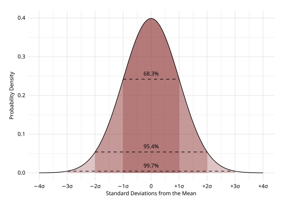
Approximately what percentage of a normal distribution lies within 2 standard deviations of the mean?
68%
99.7%
95%
90%
68-95-99.7: 68% within 1 SD, 95% within 2 SD, 99.7% within 3 SD. The two-sided 90% region is plus or minus 1.645 SD. Image: D Wells, CC BY-SA 4.0, via Wikimedia Commons.
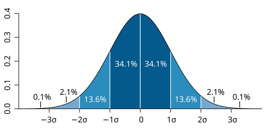
In the figure, what is the percentage of the distribution between 1 and 2 standard deviations above the mean?
13.6%
34.1%
2.1%
47.7%
The bands are 34.1% (0 to 1 sigma), 13.6% (1 to 2 sigma), 2.1% (2 to 3 sigma) and 0.1% beyond. 47.7% (34.1 + 13.6) is the area from the mean out to 2 sigma, not just the 1-2 band. Image: M. W. Toews, CC BY 2.5, via Wikimedia Commons.
A box plot has Q1 = 40 and Q3 = 60. Which value is flagged as an outlier by the 1.5 x IQR rule?
85
20
10
95
IQR = 20, so the fences are 40 - 30 = 10 and 60 + 30 = 90. 95 exceeds 90, so it is an outlier. 85 is inside the fence; 20 is above the lower fence of 10.
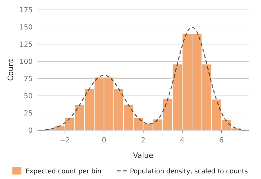
You see this histogram of customer ages for an app. What is the best next step?
Report the mean age as the typical customer age.
Investigate whether two distinct customer segments are mixed together and analyze them separately.
Remove the smaller peak as an outlier group.
Apply a log transform to make it normal.
Two peaks (bimodal) usually mean two sub-populations. The mean would land in the valley where few customers actually are. The smaller peak is real data, and a log transform does not remove bimodality. Image: Derek Jansen, CC BY 4.0, via Wikimedia Commons.
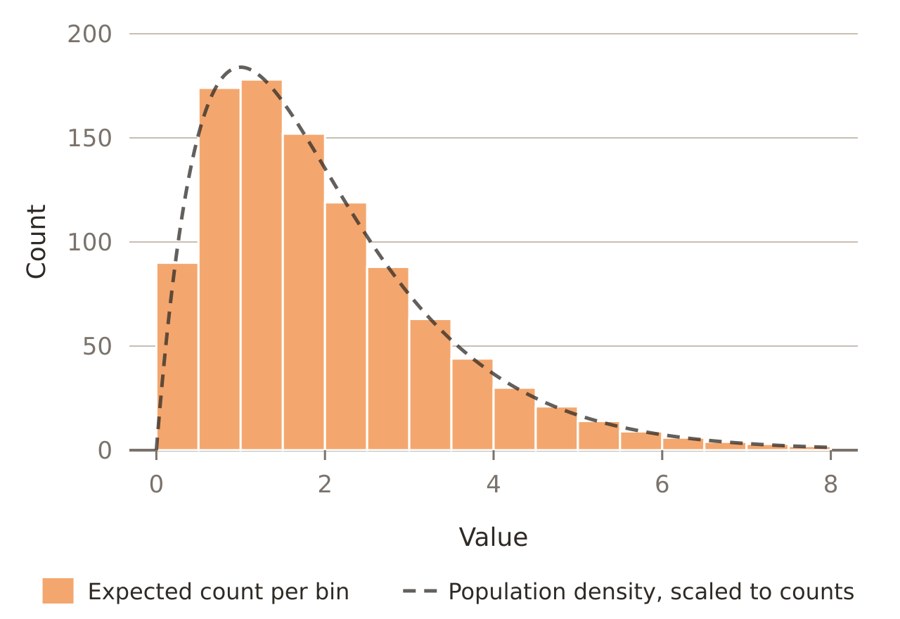
This histogram is most accurately described as:
Left-skewed, with mean greater than median
Right-skewed, with mean less than median
Right-skewed, with mean greater than median
Symmetric and unimodal
The long tail points right, so it is right (positive) skewed, and the tail pulls the mean above the median. Image: Derek Jansen, CC BY 4.0, via Wikimedia Commons.
What does a Pearson correlation of r = 0 between X and Y tell you?
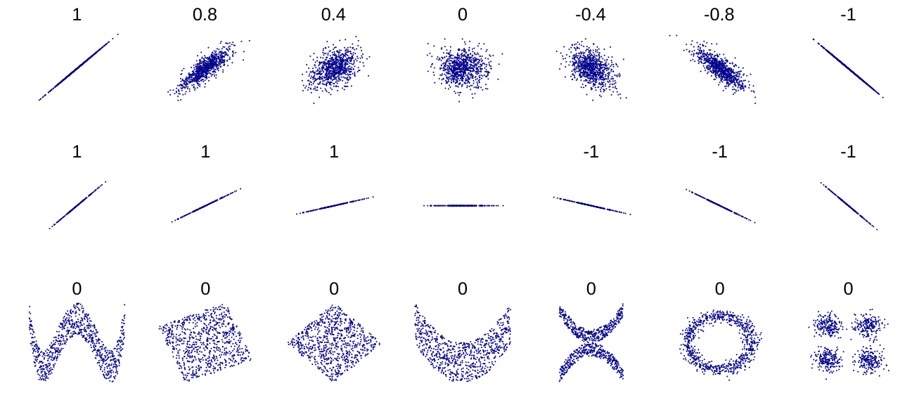
X and Y are independent.
There is no linear relationship, but a non-linear one may still exist.
Changing X never changes Y.
The regression line has a slope of 1.
r only captures linear association. Y = X squared on a symmetric range has r near 0 but is perfectly dependent. Independence implies r = 0, not the other way around.
Four datasets have identical mean, variance, correlation and regression line, yet look completely different when plotted. This is known as:
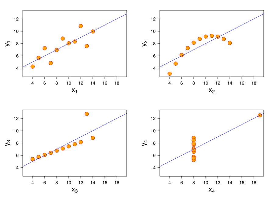
Anscombe's quartet
Simpson's paradox
The central limit theorem
Regression to the mean
Anscombe's quartet (1973) is the standard demonstration that you must plot data before trusting summary statistics. Image: Schutz and Avenue, CC BY-SA 3.0, via Wikimedia Commons.
Which correlation measure is appropriate for a monotonic but clearly curved relationship with a couple of outliers?
Pearson's correlation
Covariance
R-squared of a straight-line fit
Spearman's rank correlation
Spearman works on ranks, so it captures monotonic relationships and is resistant to outliers. Pearson assumes linearity and is outlier-sensitive; covariance is not scale-free.
A feature with a heavy right tail (positive values spanning orders of magnitude) is best prepared for linear modeling by:
Min-max scaling only
Taking the log (or log1p if zeros are present)
Replacing the tail by the mean
Subtracting the median
A log transform pulls in the long tail and often makes the relationship more linear and the residuals more even. Min-max scaling keeps the skew and is itself distorted by the extreme values.
Group A: n = 20, mean 40. Group B: n = 80, mean 70. What is the overall mean?
55
60
64
70
Weighted mean = (20 x 40 + 80 x 70)/100 = (800 + 5600)/100 = 64. The unweighted 55 ignores group sizes.
Which distribution best models the number of support tickets arriving in one hour at a roughly constant average rate?
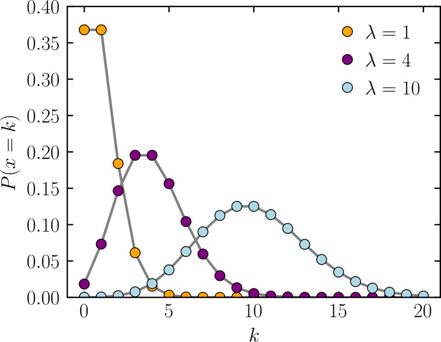
Poisson
Normal
Exponential
Uniform
Counts of independent events per fixed interval are Poisson. The exponential models the waiting time between tickets, not the count; the normal is for continuous symmetric data. Image: Skbkekas, CC BY 3.0, via Wikimedia Commons.
Which statement about the t-distribution is true?
It has lighter tails than the normal.
It is used when the sample is very large and sigma is known.
It is skewed to the right.
It has heavier tails than the normal and approaches it as degrees of freedom increase.
The t-distribution accounts for the extra uncertainty from estimating sigma with s. With many degrees of freedom it is nearly the normal.
A fair six-sided die is rolled 60 times and lands on 6 only 4 times. What does the law of large numbers imply about the next 60 rolls?
6 is now due, so it should appear more than 10 times.
6 will appear exactly 10 times to balance the earlier shortfall.
Nothing special: the long-run frequency tends to 1/6, but there is no correction owed.
The die is certainly biased.
Rolls are independent. Averages converge because later data dilute the early deviation, not because the die compensates (that is the gambler's fallacy). 4 out of 60 is not strong evidence of bias.
A disease affects 1% of people. A test is positive for 90% of the sick and also for 9% of healthy people. If you test positive, the probability you are sick is closest to:
90%
9%
50%
91%
P(sick | +) = 0.009 / (0.009 + 0.0891) = about 9.2%. The healthy majority produces far more false positives than the small sick group produces true positives. This is the base-rate fallacy.
The values 4, 8, 8, 10, 15 form a sample. What is the sample variance?
12.8
4
9
16
Mean = 9. Squared deviations: 25, 1, 1, 1, 36 = 64. Dividing by n - 1 = 4 gives 16. Dividing by n = 5 would give 12.8 (the population formula); 4 is the sample standard deviation and 9 is the mean.
Which histogram shows a left-skewed (negatively skewed) distribution?
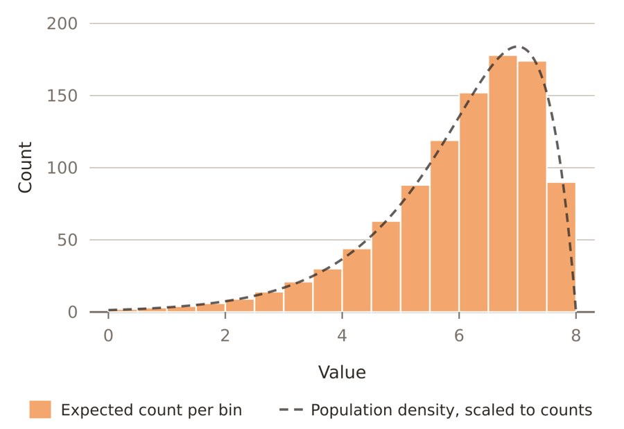
B
A
C
D
B has its long tail on the left, so it is left-skewed and its mean is below its median. A is right-skewed, C is symmetric and D is bimodal. Images: Derek Jansen, CC BY 4.0, via Wikimedia Commons.
